실습. 코비선수 데이터 분석해보기 및 테스트

Updated: August 14, 2020

https://github.com/baidoosik/kaggle-solving/tree/master/Kobe

데이터 분석

데이터 살펴보기

# import libraries
import warnings
warnings.filterwarnings('ignore')

import numpy as np
import pandas as pd
import matplotlib.pyplot as plt
import seaborn as sns

sns.set_style('whitegrid')

# display all columns
pd.set_option('display.max_columns', None)

data = pd.read_csv('data.csv')

data.head(3)
# max_columns를 설정했기 때문에 많은 column을 다 볼수 있다

	action_type	combined_shot_type	game_event_id	game_id	lat	loc_x	loc_y	lon	minutes_remaining	period	season	seconds_remaining	shot_distance	shot_made_flag	shot_type	shot_zone_area	shot_zone_basic	shot_zone_range	team_id	team_name	game_date	matchup	opponent	shot_id
0	Jump Shot	Jump Shot	10	20000012	33.9723	167	72	-118.1028	10	1	2000-01	27	18	NaN	2PT Field Goal	Right Side(R)	Mid-Range	16-24 ft.	1610612747	Los Angeles Lakers	2000-10-31	LAL @ POR	POR	1
1	Jump Shot	Jump Shot	12	20000012	34.0443	-157	0	-118.4268	10	1	2000-01	22	15	0.0	2PT Field Goal	Left Side(L)	Mid-Range	8-16 ft.	1610612747	Los Angeles Lakers	2000-10-31	LAL @ POR	POR	2
2	Jump Shot	Jump Shot	35	20000012	33.9093	-101	135	-118.3708	7	1	2000-01	45	16	1.0	2PT Field Goal	Left Side Center(LC)	Mid-Range	16-24 ft.	1610612747	Los Angeles Lakers	2000-10-31	LAL @ POR	POR	3

data.info()

<class 'pandas.core.frame.DataFrame'>
RangeIndex: 30697 entries, 0 to 30696
Data columns (total 25 columns):
 #   Column              Non-Null Count  Dtype  
---  ------              --------------  -----  
 action_type         30697 non-null  object 
 combined_shot_type  30697 non-null  object 
 game_event_id       30697 non-null  int64  
 game_id             30697 non-null  int64  
 lat                 30697 non-null  float64
 loc_x               30697 non-null  int64  
 loc_y               30697 non-null  int64  
 lon                 30697 non-null  float64
 minutes_remaining   30697 non-null  int64  
 period              30697 non-null  int64  
playoffs            30697 non-null  int64  
season              30697 non-null  object 
seconds_remaining   30697 non-null  int64  
shot_distance       30697 non-null  int64  
shot_made_flag      25697 non-null  float64
shot_type           30697 non-null  object 
shot_zone_area      30697 non-null  object 
shot_zone_basic     30697 non-null  object 
shot_zone_range     30697 non-null  object 
team_id             30697 non-null  int64  
team_name           30697 non-null  object 
game_date           30697 non-null  object 
matchup             30697 non-null  object 
opponent            30697 non-null  object 
shot_id             30697 non-null  int64  
dtypes: float64(3), int64(11), object(11)
memory usage: 5.9+ MB

# datatype -> category, object
# 데이터타입을 사용하기 좋게 변경시켜준다
data['action_type'] = data['action_type'].astype('object')
data['combined_shot_type'] = data['combined_shot_type'].astype('category')
data['game_event_id'] = data['game_event_id'].astype('category')
data['game_id'] = data['game_id'].astype('category')
data['period'] = data['period'].astype('object')
data['playoffs'] = data['playoffs'].astype('category')
data['season'] = data['season'].astype('category')
data['shot_made_flag'] = data['shot_made_flag'].astype('category')
data['shot_type'] = data['shot_type'].astype('category')
data['team_id'] = data['team_id'].astype('category')

data.set_index('shot_id', inplace = True)
# shot_id로 인덱스를 설정한다

data.head(2)

	action_type	combined_shot_type	game_event_id	game_id	lat	loc_x	loc_y	lon	minutes_remaining	period	playoffs	season	seconds_remaining	shot_distance	shot_made_flag	shot_type	shot_zone_area	shot_zone_basic	shot_zone_range	team_id	team_name	game_date	matchup	opponent
shot_id
1	Jump Shot	Jump Shot	10	20000012	33.9723	167	72	-118.1028	10	1	0	2000-01	27	18	NaN	2PT Field Goal	Right Side(R)	Mid-Range	16-24 ft.	1610612747	Los Angeles Lakers	2000-10-31	LAL @ POR	POR
2	Jump Shot	Jump Shot	12	20000012	34.0443	-157	0	-118.4268	10	1	0	2000-01	22	15	0.0	2PT Field Goal	Left Side(L)	Mid-Range	8-16 ft.	1610612747	Los Angeles Lakers	2000-10-31	LAL @ POR	POR

data.describe(include=['number'])

	lat	loc_x	loc_y	lon	minutes_remaining	seconds_remaining	shot_distance
count	30697.000000	30697.000000	30697.000000	30697.000000	30697.000000	30697.000000	30697.000000
mean	33.953192	7.110499	91.107535	-118.262690	4.885624	28.365085	13.437437
std	0.087791	110.124578	87.791361	0.110125	3.449897	17.478949	9.374189
min	33.253300	-250.000000	-44.000000	-118.519800	0.000000	0.000000	0.000000
25%	33.884300	-68.000000	4.000000	-118.337800	2.000000	13.000000	5.000000
50%	33.970300	0.000000	74.000000	-118.269800	5.000000	28.000000	15.000000
75%	34.040300	95.000000	160.000000	-118.174800	8.000000	43.000000	21.000000
max	34.088300	248.000000	791.000000	-118.021800	11.000000	59.000000	79.000000

data.describe(include=['category', 'object'])

	action_type	combined_shot_type	game_event_id	game_id	period	playoffs	season	shot_made_flag	shot_type	shot_zone_area	shot_zone_basic	shot_zone_range	team_id	team_name	game_date	matchup	opponent
count	30697	30697	30697	30697	30697	30697	30697	25697.0	30697	30697	30697	30697	30697	30697	30697	30697	30697
unique	57	6	620	1559	7	2	20	2.0	2	6	7	5	1	1	1559	74	33
top	Jump Shot	Jump Shot	2	21501228	3	0	2005-06	0.0	2PT Field Goal	Center(C)	Mid-Range	Less Than 8 ft.	1610612747	Los Angeles Lakers	2016-04-13	LAL @ SAS	SAS
freq	18880	23485	132	50	8296	26198	2318	14232.0	24271	13455	12625	9398	30697	30697	50	1020	1978

데이터 분석 및 시각화

train = data.dropna(how='any')
# any 어느 한 컬럼만 비어있어도 지워준다

def bar_chart(feature, ax=None):
    success = train[train['shot_made_flag']==1][feature].value_counts()
    fail = train[train['shot_made_flag']==0][feature].value_counts()
    df = pd.DataFrame([success, fail])
    df.index = ['Success', 'Fail']
    df.plot(kind = 'bar', stacked= True, ax=ax)

ax = plt.axes()
ax.set_title('shot made')
bar_chart('shot_made_flag',ax)
plt.show()

농구_14_0

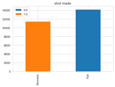
데이터에 큰 차이가 없다면 명시적으로 숫자로 확인하자

print(train['shot_made_flag'].value_counts() / len(train.index))

0.0    0.553839
1.0    0.446161
Name: shot_made_flag, dtype: float64

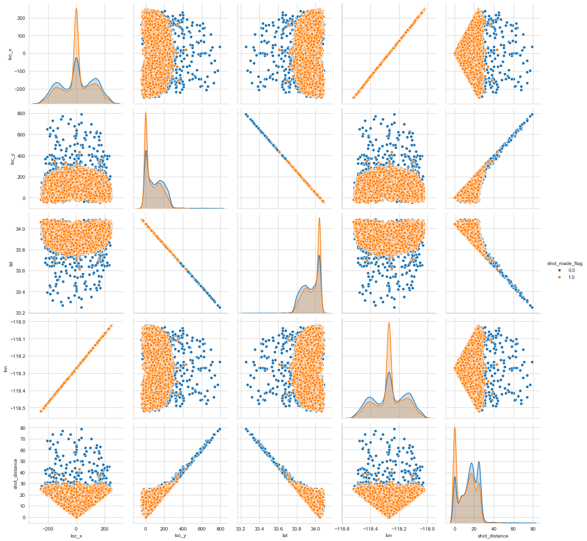
(위도, 경도),(x, y) 등 짝지었을 때 의미있는 데이터 Seaborn 라이브러리의 pairplot을 이용한 시각화

sns.pairplot(train, vars=['loc_x','loc_y','lat','lon','shot_distance'], hue='shot_made_flag', size=3)
plt.show()

농구_18_0

Category 데이터의 항목이 많은 경우 stack방식이 아닌 Seaborn 라이브러리의 countplot() 함수를 이용

def count_plot(column, ax):
    sns.countplot(x=column, hue='shot_made_flag', data=train, ax=ax)

f, axrr = plt.subplots(8, figsize=(15,30))

categorical_data=['combined_shot_type','season','period','playoffs','shot_type','shot_zone_area','shot_zone_basic','shot_zone_range']

for idx, category_data in enumerate(categorical_data,0):
    count_plot(category_data, axrr[idx])
    axrr[idx].set_title(category_data)
    
plt.tight_layout()
plt.show

<function matplotlib.pyplot.show(*args, **kw)>

농구_21_1

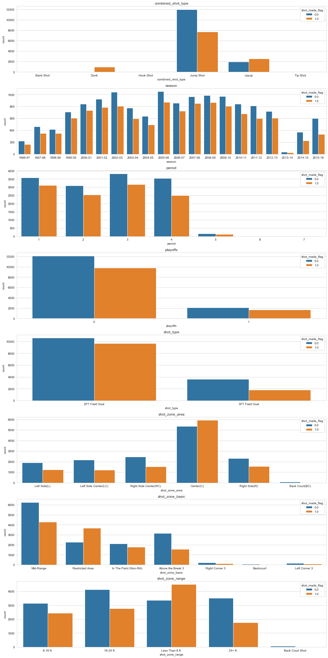
값이 비슷해 보일 때는 명시적으로 숫자로 보자

def print_probability(column):
    print(train[train['shot_made_flag']==1][column].value_counts()/(train[train['shot_made_flag']==1][column].value_counts()+train[train['shot_made_flag']==0][column].value_counts()))

for categoty_data in categorical_data:
    print(print_probability(categoty_data))

Bank Shot    0.791667
Dunk         0.928030
Hook Shot    0.535433
Jump Shot    0.391071
Layup        0.565093
Tip Shot     0.348684
Name: combined_shot_type, dtype: float64
None
1996-97    0.422977
1997-98    0.430864
1998-99    0.458824
1999-00    0.460366
2000-01    0.466667
2001-02    0.458431
2002-03    0.436285
2003-04    0.433260
2004-05    0.436557
2005-06    0.453742
2006-07    0.457885
2007-08    0.468389
2008-09    0.467855
2009-10    0.453725
2010-11    0.446417
2011-12    0.425847
2012-13    0.457831
2013-14    0.406780
2014-15    0.376054
2015-16    0.356223
Name: season, dtype: float64
None
1    0.465672
2    0.448802
3    0.453442
4    0.413702
5    0.442857
6    0.466667
7    0.428571
Name: period, dtype: float64
None
0    0.446420
1    0.444651
Name: playoffs, dtype: float64
None
2PT Field Goal    0.477348
3PT Field Goal    0.329268
Name: shot_type, dtype: float64
None
Back Court(BC)           0.013889
Center(C)                0.525556
Left Side Center(LC)     0.361177
Left Side(L)             0.396871
Right Side Center(RC)    0.382567
Right Side(R)            0.401658
Name: shot_zone_area, dtype: float64
None
Above the Break 3        0.329237
Backcourt                0.016667
In The Paint (Non-RA)    0.454381
Left Corner 3            0.370833
Mid-Range                0.406286
Restricted Area          0.618004
Right Corner 3           0.339339
Name: shot_zone_basic, dtype: float64
None
16-24 ft.          0.401766
24+ ft.            0.332513
8-16 ft.           0.435484
Back Court Shot    0.013889
Less Than 8 ft.    0.573120
Name: shot_zone_range, dtype: float64
None

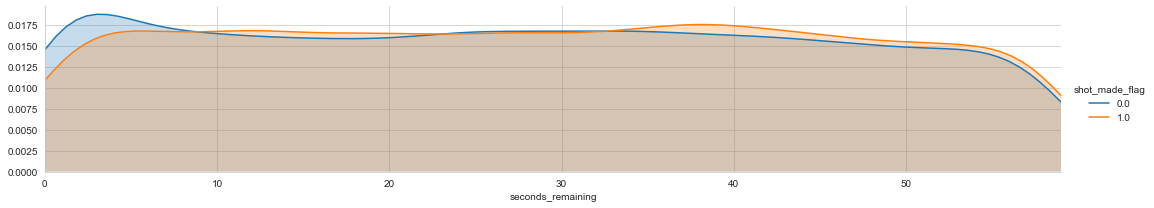
continuous 한 데이터들 시각화 facet_grid를 이용

def draw_facetgrid(feature):
    facet = sns.FacetGrid(train, hue='shot_made_flag',aspect=5)
    facet.map(sns.kdeplot, feature, shade=True)
    facet.set(xlim=(0, train[feature].max()))
    # survived 라벨을 표시.
    facet.add_legend()
    plt.show()

draw_facetgrid('minutes_remaining')

농구_27_0

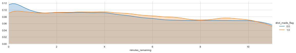
draw_facetgrid('seconds_remaining')

농구_28_0

group_by 함수를 이용해 두개 column을 합쳐서 분석하기

train['shot_made_flag'] = train['shot_made_flag'].astype('int64')

train.groupby(['season','combined_shot_type'])['shot_made_flag'].sum()/(train.groupby(['season','combined_shot_type'])['shot_made_flag'].count())

season   combined_shot_type
1996-97  Bank Shot                  NaN
         Dunk                  0.947368
         Hook Shot                  NaN
         Jump Shot             0.380567
         Layup                 0.450450
                                 ...   
2015-16  Dunk                  1.000000
         Hook Shot             0.272727
         Jump Shot             0.327711
         Layup                 0.623529
         Tip Shot                   NaN
Name: shot_made_flag, Length: 120, dtype: float64

Feature Engineering

Data cleaning

Featureing 단계에서 필요없는 데이터들을 삭제 작업을 시작하기 전에 정리

data_cp = data.copy()
target = data_cp['shot_made_flag'].copy()

# 코비는 하나의 팀에서만 활동했기때문에 team_id, team_name이 의미없다
data_cp.drop('team_id', axis=1, inplace=True)
data_cp.drop('team_name', axis=1, inplace=True)

# lat, lon -> loc_x, loc_y 로 대치가능
data_cp.drop('lat', axis=1, inplace=True)
data_cp.drop('lon', axis=1, inplace=True)

# game_id, game_event_id are independent
data_cp.drop('game_id', axis=1, inplace=True)
data_cp.drop('game_event_id', axis=1, inplace=True)

data_cp.drop('shot_made_flag', axis=1, inplace= True)

data_cp.head(2)

	action_type	combined_shot_type	loc_x	loc_y	minutes_remaining	period	playoffs	season	seconds_remaining	shot_distance	shot_type	shot_zone_area	shot_zone_basic	shot_zone_range	game_date	matchup	opponent
shot_id
1	Jump Shot	Jump Shot	167	72	10	1	0	2000-01	27	18	2PT Field Goal	Right Side(R)	Mid-Range	16-24 ft.	2000-10-31	LAL @ POR	POR
2	Jump Shot	Jump Shot	-157	0	10	1	0	2000-01	22	15	2PT Field Goal	Left Side(L)	Mid-Range	8-16 ft.	2000-10-31	LAL @ POR	POR

Data Transformation

의미 있는 데이터 즉 feature로 변형
시각화를 통해 5초 이하의 시간이 남았을 때 특설을 찾음

# 시간 그래프를 보면 시간이 적게 남았을 때 안들어갈 확률이 높음
data_cp['seconds_from_period_end'] = 60 * data_cp['minutes_remaining'] + data_cp['seconds_remaining']

data_cp['last_5_sec_in_period'] = data_cp['seconds_from_period_end']<5

# 사용한 시간 컬럼을 지워준다
data_cp.drop('minutes_remaining', axis=1, inplace=True)
data_cp.drop('seconds_remaining', axis=1, inplace=True)
data_cp.drop('seconds_from_period_end', axis=1, inplace=True)

## home, away mapping
data_cp['home_away'] = data_cp['matchup'].str.contains('vs').astype('int')
data_cp.drop('matchup', axis=1, inplace=True)

data_cp.head(1)

	action_type	combined_shot_type	loc_x	loc_y	period	playoffs	season	shot_distance	shot_type	shot_zone_area	shot_zone_basic	shot_zone_range	game_date	opponent	last_5_sec_in_period	home_away
shot_id
1	Jump Shot	Jump Shot	167	72	1	0	2000-01	18	2PT Field Goal	Right Side(R)	Mid-Range	16-24 ft.	2000-10-31	POR	False	0

# game data 년/월/일

data_cp['game_date'] = pd.to_datetime(data_cp['game_date'])

data_cp['game_year'] = data_cp['game_date'].dt.year
data_cp['game_month'] = data_cp['game_date'].dt.month

data_cp.drop('game_date', axis = 1, inplace=True)

data_cp.head(2)

	action_type	combined_shot_type	loc_x	loc_y	period	playoffs	season	shot_distance	shot_type	shot_zone_area	shot_zone_basic	shot_zone_range	opponent	last_5_sec_in_period	home_away	game_year	game_month
shot_id
1	Jump Shot	Jump Shot	167	72	1	0	2000-01	18	2PT Field Goal	Right Side(R)	Mid-Range	16-24 ft.	POR	False	0	2000	10
2	Jump Shot	Jump Shot	-157	0	1	0	2000-01	15	2PT Field Goal	Left Side(L)	Mid-Range	8-16 ft.	POR	False	0	2000	10

# loc_x, loc_y binding 25 단위로

data_cp['loc_x'] = pd.cut(data_cp['loc_x'],25)
data_cp['loc_y'] = pd.cut(data_cp['loc_y'],25)

# 1~2개의 데이터는 의미가 없다
# 인덱싱
data_cp.action_type.value_counts()

Jump Shot                             18880
Layup Shot                             2567
Driving Layup Shot                     1978
Turnaround Jump Shot                   1057
Fadeaway Jump Shot                     1048
Running Jump Shot                       926
Pullup Jump shot                        476
Turnaround Fadeaway shot                439
Slam Dunk Shot                          411
Reverse Layup Shot                      395
Jump Bank Shot                          333
Driving Dunk Shot                       310
Dunk Shot                               262
Tip Shot                                182
Alley Oop Dunk Shot                     122
Step Back Jump shot                     118
Floating Jump shot                      114
Driving Reverse Layup Shot               97
Hook Shot                                84
Driving Finger Roll Shot                 82
Alley Oop Layup shot                     80
Reverse Dunk Shot                        75
Running Layup Shot                       72
Turnaround Bank shot                     71
Driving Finger Roll Layup Shot           69
Driving Slam Dunk Shot                   48
Running Bank shot                        48
Running Hook Shot                        41
Finger Roll Layup Shot                   33
Fadeaway Bank shot                       31
Driving Jump shot                        28
Finger Roll Shot                         28
Jump Hook Shot                           24
Running Dunk Shot                        19
Reverse Slam Dunk Shot                   16
Putback Layup Shot                       15
Follow Up Dunk Shot                      15
Driving Hook Shot                        14
Turnaround Hook Shot                     14
Pullup Bank shot                         12
Running Reverse Layup Shot               11
Running Finger Roll Layup Shot            6
Cutting Layup Shot                        6
Hook Bank Shot                            5
Driving Bank shot                         5
Driving Floating Jump Shot                5
Putback Dunk Shot                         5
Running Finger Roll Shot                  4
Running Pull-Up Jump Shot                 4
Turnaround Finger Roll Shot               2
Tip Layup Shot                            2
Putback Slam Dunk Shot                    2
Running Tip Shot                          2
Running Slam Dunk Shot                    1
Cutting Finger Roll Layup Shot            1
Driving Floating Bank Jump Shot           1
Turnaround Fadeaway Bank Jump Shot        1
Name: action_type, dtype: int64

rare_action_types = data_cp['action_type'].value_counts().sort_values().index.values[:20]
rare_action_types

array(['Turnaround Fadeaway Bank Jump Shot', 'Running Slam Dunk Shot',
       'Driving Floating Bank Jump Shot',
       'Cutting Finger Roll Layup Shot', 'Running Tip Shot',
       'Putback Slam Dunk Shot', 'Tip Layup Shot',
       'Turnaround Finger Roll Shot', 'Running Pull-Up Jump Shot',
       'Running Finger Roll Shot', 'Putback Dunk Shot',
       'Driving Floating Jump Shot', 'Driving Bank shot',
       'Hook Bank Shot', 'Cutting Layup Shot',
       'Running Finger Roll Layup Shot', 'Running Reverse Layup Shot',
       'Pullup Bank shot', 'Turnaround Hook Shot', 'Driving Hook Shot'],
      dtype=object)

data_cp.loc[data_cp['action_type'].isin(rare_action_types), 'action_type'] = 'Other'

data_cp.head(2)

	action_type	combined_shot_type	loc_x	loc_y	period	playoffs	season	shot_distance	shot_type	shot_zone_area	shot_zone_basic	shot_zone_range	opponent	last_5_sec_in_period	home_away	game_year	game_month
shot_id
1	Jump Shot	Jump Shot	(148.4, 168.32]	(56.2, 89.6]	1	0	2000-01	18	2PT Field Goal	Right Side(R)	Mid-Range	16-24 ft.	POR	False	0	2000	10
2	Jump Shot	Jump Shot	(-170.32, -150.4]	(-10.6, 22.8]	1	0	2000-01	15	2PT Field Goal	Left Side(L)	Mid-Range	8-16 ft.	POR	False	0	2000	10

categorial_cols = {'action_type', 'combined_shot_type','period', 'season','shot_type','shot_zone_area', 'shot_zone_basic','shot_zone_range','game_year','game_month','opponent','loc_x','loc_y'}

pd.get_dummies?

Convert categorical variable into dummy/indicator variables.

Parameters
----------
data : array-like, Series, or DataFrame
    Data of which to get dummy indicators.
prefix : str, list of str, or dict of str, default None
    String to append DataFrame column names.
    Pass a list with length equal to the number of columns
    when calling get_dummies on a DataFrame. Alternatively, `prefix`
    can be a dictionary mapping column names to prefixes.
prefix_sep : str, default '_'
    If appending prefix, separator/delimiter to use. Or pass a
    list or dictionary as with `prefix`.
dummy_na : bool, default False
    Add a column to indicate NaNs, if False NaNs are ignored.
columns : list-like, default None
    Column names in the DataFrame to be encoded.
    If `columns` is None then all the columns with
    `object` or `category` dtype will be converted.
sparse : bool, default False
    Whether the dummy-encoded columns should be backed by
    a :class:`SparseArray` (True) or a regular NumPy array (False).
drop_first : bool, default False
    Whether to get k-1 dummies out of k categorical levels by removing the
    first level.
dtype : dtype, default np.uint8
    Data type for new columns. Only a single dtype is allowed.

    .. versionadded:: 0.23.0

Returns
-------
DataFrame
    Dummy-coded data.

See Also
--------
Series.str.get_dummies : Convert Series to dummy codes.

Examples
--------
>>> s = pd.Series(list('abca'))

>>> pd.get_dummies(s)
   a  b  c
0  1  0  0
1  0  1  0
2  0  0  1
3  1  0  0

>>> s1 = ['a', 'b', np.nan]

>>> pd.get_dummies(s1)
   a  b
0  1  0
1  0  1
2  0  0

>>> pd.get_dummies(s1, dummy_na=True)
   a  b  NaN
0  1  0    0
1  0  1    0
2  0  0    1

>>> df = pd.DataFrame({'A': ['a', 'b', 'a'], 'B': ['b', 'a', 'c'],
...                    'C': [1, 2, 3]})

>>> pd.get_dummies(df, prefix=['col1', 'col2'])
   C  col1_a  col1_b  col2_a  col2_b  col2_c
0  1       1       0       0       1       0
1  2       0       1       1       0       0
2  3       1       0       0       0       1

>>> pd.get_dummies(pd.Series(list('abcaa')))
   a  b  c
0  1  0  0
1  0  1  0
2  0  0  1
3  1  0  0
4  1  0  0

>>> pd.get_dummies(pd.Series(list('abcaa')), drop_first=True)
   b  c
0  0  0
1  1  0
2  0  1
3  0  0
4  0  0

>>> pd.get_dummies(pd.Series(list('abc')), dtype=float)
     a    b    c
0  1.0  0.0  0.0
1  0.0  1.0  0.0
2  0.0  0.0  1.0
[1;31mFile:[0m      c:\users\user\anaconda3\lib\site-packages\pandas\core\reshape\reshape.py
[1;31mType:[0m      function

data_cp.join?

Join columns of another DataFrame.

Join columns with `other` DataFrame either on index or on a key
column. Efficiently join multiple DataFrame objects by index at once by
passing a list.

Parameters
----------
other : DataFrame, Series, or list of DataFrame
    Index should be similar to one of the columns in this one. If a
    Series is passed, its name attribute must be set, and that will be
    used as the column name in the resulting joined DataFrame.
on : str, list of str, or array-like, optional
    Column or index level name(s) in the caller to join on the index
    in `other`, otherwise joins index-on-index. If multiple
    values given, the `other` DataFrame must have a MultiIndex. Can
    pass an array as the join key if it is not already contained in
    the calling DataFrame. Like an Excel VLOOKUP operation.
how : {'left', 'right', 'outer', 'inner'}, default 'left'
    How to handle the operation of the two objects.

    * left: use calling frame's index (or column if on is specified)
    * right: use `other`'s index.
    * outer: form union of calling frame's index (or column if on is
      specified) with `other`'s index, and sort it.
      lexicographically.
    * inner: form intersection of calling frame's index (or column if
      on is specified) with `other`'s index, preserving the order
      of the calling's one.
lsuffix : str, default ''
    Suffix to use from left frame's overlapping columns.
rsuffix : str, default ''
    Suffix to use from right frame's overlapping columns.
sort : bool, default False
    Order result DataFrame lexicographically by the join key. If False,
    the order of the join key depends on the join type (how keyword).

Returns
-------
DataFrame
    A dataframe containing columns from both the caller and `other`.

See Also
--------
DataFrame.merge : For column(s)-on-columns(s) operations.

Notes
-----
Parameters `on`, `lsuffix`, and `rsuffix` are not supported when
passing a list of `DataFrame` objects.

Support for specifying index levels as the `on` parameter was added
in version 0.23.0.

Examples
--------
>>> df = pd.DataFrame({'key': ['K0', 'K1', 'K2', 'K3', 'K4', 'K5'],
...                    'A': ['A0', 'A1', 'A2', 'A3', 'A4', 'A5']})

>>> df
  key   A
0  K0  A0
1  K1  A1
2  K2  A2
3  K3  A3
4  K4  A4
5  K5  A5

>>> other = pd.DataFrame({'key': ['K0', 'K1', 'K2'],
...                       'B': ['B0', 'B1', 'B2']})

>>> other
  key   B
0  K0  B0
1  K1  B1
2  K2  B2

Join DataFrames using their indexes.

>>> df.join(other, lsuffix='_caller', rsuffix='_other')
  key_caller   A key_other    B
0         K0  A0        K0   B0
1         K1  A1        K1   B1
2         K2  A2        K2   B2
3         K3  A3       NaN  NaN
4         K4  A4       NaN  NaN
5         K5  A5       NaN  NaN

If we want to join using the key columns, we need to set key to be
the index in both `df` and `other`. The joined DataFrame will have
key as its index.

>>> df.set_index('key').join(other.set_index('key'))
      A    B
key
K0   A0   B0
K1   A1   B1
K2   A2   B2
K3   A3  NaN
K4   A4  NaN
K5   A5  NaN

Another option to join using the key columns is to use the `on`
parameter. DataFrame.join always uses `other`'s index but we can use
any column in `df`. This method preserves the original DataFrame's
index in the result.

>>> df.join(other.set_index('key'), on='key')
  key   A    B
0  K0  A0   B0
1  K1  A1   B1
2  K2  A2   B2
3  K3  A3  NaN
4  K4  A4  NaN
5  K5  A5  NaN
[1;31mFile:[0m      c:\users\user\anaconda3\lib\site-packages\pandas\core\frame.py
[1;31mType:[0m      method

for column in categorial_cols:
    # cataegorical variable 을 dummy변수로 바꾸어준다
    dummies = pd.get_dummies(data_cp[column])
    dummies = dummies.add_prefix("{}#".format(column))
    data_cp.drop(column, axis=1, inplace=True)
    # join 은 두 데이터 프레임을 합친다
    data_cp = data_cp.join(dummies)

data_cp

	playoffs	shot_distance	last_5_sec_in_period	home_away	shot_zone_basic#Above the Break 3	shot_zone_basic#Backcourt	shot_zone_basic#In The Paint (Non-RA)	shot_zone_basic#Left Corner 3	shot_zone_basic#Mid-Range	shot_zone_basic#Restricted Area	shot_zone_basic#Right Corner 3	season#1996-97	season#1997-98	season#1998-99	season#1999-00	season#2000-01	season#2001-02	season#2002-03	season#2003-04	season#2004-05	season#2005-06	season#2006-07	season#2007-08	season#2008-09	season#2009-10	season#2010-11	season#2011-12	season#2012-13	season#2013-14	season#2014-15	season#2015-16	shot_zone_area#Back Court(BC)	shot_zone_area#Center(C)	shot_zone_area#Left Side Center(LC)	shot_zone_area#Left Side(L)	shot_zone_area#Right Side Center(RC)	shot_zone_area#Right Side(R)	game_year#1996	game_year#1997	game_year#1998	game_year#1999	game_year#2000	game_year#2001	game_year#2002	game_year#2003	game_year#2004	game_year#2005	game_year#2006	game_year#2007	game_year#2008	game_year#2009	game_year#2010	game_year#2011	game_year#2012	game_year#2013	game_year#2014	game_year#2015	game_year#2016	shot_type#2PT Field Goal	shot_type#3PT Field Goal	game_month#1	game_month#2	game_month#3	game_month#4	game_month#5	game_month#6	game_month#10	game_month#11	game_month#12	loc_x#(-250.498, -230.08]	loc_x#(-230.08, -210.16]	loc_x#(-210.16, -190.24]	loc_x#(-190.24, -170.32]	loc_x#(-170.32, -150.4]	loc_x#(-150.4, -130.48]	loc_x#(-130.48, -110.56]	loc_x#(-110.56, -90.64]	loc_x#(-90.64, -70.72]	loc_x#(-70.72, -50.8]	loc_x#(-50.8, -30.88]	loc_x#(-30.88, -10.96]	loc_x#(-10.96, 8.96]	loc_x#(8.96, 28.88]	loc_x#(28.88, 48.8]	loc_x#(48.8, 68.72]	loc_x#(68.72, 88.64]	loc_x#(88.64, 108.56]	loc_x#(108.56, 128.48]	loc_x#(128.48, 148.4]	loc_x#(148.4, 168.32]	loc_x#(168.32, 188.24]	loc_x#(188.24, 208.16]	loc_x#(208.16, 228.08]	loc_x#(228.08, 248.0]	combined_shot_type#Bank Shot	combined_shot_type#Dunk	combined_shot_type#Hook Shot	combined_shot_type#Jump Shot	combined_shot_type#Layup	combined_shot_type#Tip Shot	loc_y#(-44.835, -10.6]	loc_y#(-10.6, 22.8]	loc_y#(22.8, 56.2]	loc_y#(56.2, 89.6]	loc_y#(89.6, 123.0]	loc_y#(123.0, 156.4]	loc_y#(156.4, 189.8]	loc_y#(189.8, 223.2]	loc_y#(223.2, 256.6]	loc_y#(256.6, 290.0]	loc_y#(290.0, 323.4]	loc_y#(323.4, 356.8]	loc_y#(356.8, 390.2]	loc_y#(390.2, 423.6]	loc_y#(423.6, 457.0]	loc_y#(457.0, 490.4]	loc_y#(490.4, 523.8]	loc_y#(523.8, 557.2]	loc_y#(557.2, 590.6]	loc_y#(590.6, 624.0]	loc_y#(624.0, 657.4]	loc_y#(657.4, 690.8]	loc_y#(690.8, 724.2]	loc_y#(724.2, 757.6]	loc_y#(757.6, 791.0]	period#1	period#2	period#3	period#4	period#5	period#6	period#7	opponent#ATL	opponent#BKN	opponent#BOS	opponent#CHA	opponent#CHI	opponent#CLE	opponent#DAL	opponent#DEN	opponent#DET	opponent#GSW	opponent#HOU	opponent#IND	opponent#LAC	opponent#MEM	opponent#MIA	opponent#MIL	opponent#MIN	opponent#NJN	opponent#NOH	opponent#NOP	opponent#NYK	opponent#OKC	opponent#ORL	opponent#PHI	opponent#PHX	opponent#POR	opponent#SAC	opponent#SAS	opponent#SEA	opponent#TOR	opponent#UTA	opponent#VAN	opponent#WAS	action_type#Alley Oop Dunk Shot	action_type#Alley Oop Layup shot	action_type#Driving Dunk Shot	action_type#Driving Finger Roll Layup Shot	action_type#Driving Finger Roll Shot	action_type#Driving Jump shot	action_type#Driving Layup Shot	action_type#Driving Reverse Layup Shot	action_type#Driving Slam Dunk Shot	action_type#Dunk Shot	action_type#Fadeaway Bank shot	action_type#Fadeaway Jump Shot	action_type#Finger Roll Layup Shot	action_type#Finger Roll Shot	action_type#Floating Jump shot	action_type#Follow Up Dunk Shot	action_type#Hook Shot	action_type#Jump Bank Shot	action_type#Jump Hook Shot	action_type#Jump Shot	action_type#Layup Shot	action_type#Other	action_type#Pullup Jump shot	action_type#Putback Layup Shot	action_type#Reverse Dunk Shot	action_type#Reverse Layup Shot	action_type#Reverse Slam Dunk Shot	action_type#Running Bank shot	action_type#Running Dunk Shot	action_type#Running Hook Shot	action_type#Running Jump Shot	action_type#Running Layup Shot	action_type#Slam Dunk Shot	action_type#Step Back Jump shot	action_type#Tip Shot	action_type#Turnaround Bank shot	action_type#Turnaround Fadeaway shot	action_type#Turnaround Jump Shot	shot_zone_range#16-24 ft.	shot_zone_range#24+ ft.	shot_zone_range#8-16 ft.	shot_zone_range#Back Court Shot	shot_zone_range#Less Than 8 ft.
shot_id
1	0	18	False	0	0	0	0	0	1	0	0	0	0	0	0	1	0	0	0	0	0	0	0	0	0	0	0	0	0	0	0	0	0	0	0	0	1	0	0	0	0	1	0	0	0	0	0	0	0	0	0	0	0	0	0	0	0	0	1	0	0	0	0	0	0	0	1	0	0	0	0	0	0	0	0	0	0	0	0	0	0	0	0	0	0	0	0	0	0	1	0	0	0	0	0	0	0	1	0	0	0	0	0	1	0	0	0	0	0	0	0	0	0	0	0	0	0	0	0	0	0	0	0	0	0	1	0	0	0	0	0	0	0	0	0	0	0	0	0	0	0	0	0	0	0	0	0	0	0	0	0	0	0	0	0	0	0	1	0	0	0	0	0	0	0	0	0	0	0	0	0	0	0	0	0	0	0	0	0	0	0	0	0	0	1	0	0	0	0	0	0	0	0	0	0	0	0	0	0	0	0	0	0	1	0	0	0	0
2	0	15	False	0	0	0	0	0	1	0	0	0	0	0	0	1	0	0	0	0	0	0	0	0	0	0	0	0	0	0	0	0	0	0	1	0	0	0	0	0	0	1	0	0	0	0	0	0	0	0	0	0	0	0	0	0	0	0	1	0	0	0	0	0	0	0	1	0	0	0	0	0	0	1	0	0	0	0	0	0	0	0	0	0	0	0	0	0	0	0	0	0	0	0	0	0	0	1	0	0	0	1	0	0	0	0	0	0	0	0	0	0	0	0	0	0	0	0	0	0	0	0	0	0	0	1	0	0	0	0	0	0	0	0	0	0	0	0	0	0	0	0	0	0	0	0	0	0	0	0	0	0	0	0	0	0	0	1	0	0	0	0	0	0	0	0	0	0	0	0	0	0	0	0	0	0	0	0	0	0	0	0	0	0	1	0	0	0	0	0	0	0	0	0	0	0	0	0	0	0	0	0	0	0	0	1	0	0
3	0	16	False	0	0	0	0	0	1	0	0	0	0	0	0	1	0	0	0	0	0	0	0	0	0	0	0	0	0	0	0	0	0	1	0	0	0	0	0	0	0	1	0	0	0	0	0	0	0	0	0	0	0	0	0	0	0	0	1	0	0	0	0	0	0	0	1	0	0	0	0	0	0	0	0	0	1	0	0	0	0	0	0	0	0	0	0	0	0	0	0	0	0	0	0	0	0	1	0	0	0	0	0	0	0	1	0	0	0	0	0	0	0	0	0	0	0	0	0	0	0	0	0	0	0	1	0	0	0	0	0	0	0	0	0	0	0	0	0	0	0	0	0	0	0	0	0	0	0	0	0	0	0	0	0	0	0	1	0	0	0	0	0	0	0	0	0	0	0	0	0	0	0	0	0	0	0	0	0	0	0	0	0	0	1	0	0	0	0	0	0	0	0	0	0	0	0	0	0	0	0	0	0	1	0	0	0	0
4	0	22	False	0	0	0	0	0	1	0	0	0	0	0	0	1	0	0	0	0	0	0	0	0	0	0	0	0	0	0	0	0	0	0	0	1	0	0	0	0	0	1	0	0	0	0	0	0	0	0	0	0	0	0	0	0	0	0	1	0	0	0	0	0	0	0	1	0	0	0	0	0	0	0	0	0	0	0	0	0	0	0	0	0	0	0	0	0	1	0	0	0	0	0	0	0	0	1	0	0	0	0	0	0	0	0	1	0	0	0	0	0	0	0	0	0	0	0	0	0	0	0	0	0	0	1	0	0	0	0	0	0	0	0	0	0	0	0	0	0	0	0	0	0	0	0	0	0	0	0	0	0	0	0	0	0	0	1	0	0	0	0	0	0	0	0	0	0	0	0	0	0	0	0	0	0	0	0	0	0	0	0	0	0	1	0	0	0	0	0	0	0	0	0	0	0	0	0	0	0	0	0	0	1	0	0	0	0
5	0	0	False	0	0	0	0	0	0	1	0	0	0	0	0	1	0	0	0	0	0	0	0	0	0	0	0	0	0	0	0	0	1	0	0	0	0	0	0	0	0	1	0	0	0	0	0	0	0	0	0	0	0	0	0	0	0	0	1	0	0	0	0	0	0	0	1	0	0	0	0	0	0	0	0	0	0	0	0	0	0	1	0	0	0	0	0	0	0	0	0	0	0	0	0	1	0	0	0	0	0	1	0	0	0	0	0	0	0	0	0	0	0	0	0	0	0	0	0	0	0	0	0	0	0	0	1	0	0	0	0	0	0	0	0	0	0	0	0	0	0	0	0	0	0	0	0	0	0	0	0	0	0	0	0	0	0	1	0	0	0	0	0	0	0	0	0	1	0	0	0	0	0	0	0	0	0	0	0	0	0	0	0	0	0	0	0	0	0	0	0	0	0	0	0	0	0	0	0	0	0	0	0	0	0	0	0	1
...	...	...	...	...	...	...	...	...	...	...	...	...	...	...	...	...	...	...	...	...	...	...	...	...	...	...	...	...	...	...	...	...	...	...	...	...	...	...	...	...	...	...	...	...	...	...	...	...	...	...	...	...	...	...	...	...	...	...	...	...	...	...	...	...	...	...	...	...	...	...	...	...	...	...	...	...	...	...	...	...	...	...	...	...	...	...	...	...	...	...	...	...	...	...	...	...	...	...	...	...	...	...	...	...	...	...	...	...	...	...	...	...	...	...	...	...	...	...	...	...	...	...	...	...	...	...	...	...	...	...	...	...	...	...	...	...	...	...	...	...	...	...	...	...	...	...	...	...	...	...	...	...	...	...	...	...	...	...	...	...	...	...	...	...	...	...	...	...	...	...	...	...	...	...	...	...	...	...	...	...	...	...	...	...	...	...	...	...	...	...	...	...	...	...	...	...	...	...	...	...	...	...	...	...	...	...	...	...
30693	1	4	False	1	0	0	1	0	0	0	0	0	0	0	1	0	0	0	0	0	0	0	0	0	0	0	0	0	0	0	0	0	1	0	0	0	0	0	0	0	0	1	0	0	0	0	0	0	0	0	0	0	0	0	0	0	0	0	1	0	0	0	0	0	0	1	0	0	0	0	0	0	0	0	0	0	0	0	0	0	0	1	0	0	0	0	0	0	0	0	0	0	0	0	0	0	0	1	0	0	0	0	1	0	0	0	0	0	0	0	0	0	0	0	0	0	0	0	0	0	0	0	0	0	0	0	0	0	1	0	0	0	0	0	0	0	0	0	0	0	0	0	0	1	0	0	0	0	0	0	0	0	0	0	0	0	0	0	0	0	0	0	0	0	0	0	0	0	0	0	0	0	0	0	0	0	0	0	0	0	0	0	0	0	1	0	0	0	0	0	0	0	0	0	0	0	0	0	0	0	0	0	0	0	0	0	0	1
30694	1	0	False	1	0	0	0	0	0	1	0	0	0	0	1	0	0	0	0	0	0	0	0	0	0	0	0	0	0	0	0	0	1	0	0	0	0	0	0	0	0	1	0	0	0	0	0	0	0	0	0	0	0	0	0	0	0	0	1	0	0	0	0	0	0	1	0	0	0	0	0	0	0	0	0	0	0	0	0	0	0	1	0	0	0	0	0	0	0	0	0	0	0	0	0	0	0	0	0	1	0	1	0	0	0	0	0	0	0	0	0	0	0	0	0	0	0	0	0	0	0	0	0	0	0	0	0	0	1	0	0	0	0	0	0	0	0	0	0	0	0	0	0	1	0	0	0	0	0	0	0	0	0	0	0	0	0	0	0	0	0	0	0	0	0	0	0	0	0	0	0	0	0	0	0	0	0	0	0	0	0	0	0	0	0	0	0	0	0	0	0	0	0	0	0	0	0	0	0	1	0	0	0	0	0	0	0	1
30695	1	21	False	1	0	0	0	0	1	0	0	0	0	0	1	0	0	0	0	0	0	0	0	0	0	0	0	0	0	0	0	0	0	1	0	0	0	0	0	0	0	1	0	0	0	0	0	0	0	0	0	0	0	0	0	0	0	0	1	0	0	0	0	0	0	1	0	0	0	0	0	0	0	0	1	0	0	0	0	0	0	0	0	0	0	0	0	0	0	0	0	0	0	0	0	0	0	1	0	0	0	0	0	0	0	0	1	0	0	0	0	0	0	0	0	0	0	0	0	0	0	0	0	0	0	0	0	0	1	0	0	0	0	0	0	0	0	0	0	0	0	0	0	1	0	0	0	0	0	0	0	0	0	0	0	0	0	0	0	0	0	0	0	0	0	0	0	0	0	0	0	0	0	0	0	0	0	0	0	0	0	0	0	0	0	0	0	0	0	0	0	0	0	0	0	1	0	0	0	0	0	0	0	1	0	0	0	0
30696	1	26	False	1	1	0	0	0	0	0	0	0	0	0	1	0	0	0	0	0	0	0	0	0	0	0	0	0	0	0	0	0	1	0	0	0	0	0	0	0	0	1	0	0	0	0	0	0	0	0	0	0	0	0	0	0	0	0	0	1	0	0	0	0	0	1	0	0	0	0	0	0	0	0	0	0	0	0	0	0	0	0	0	1	0	0	0	0	0	0	0	0	0	0	0	0	0	1	0	0	0	0	0	0	0	0	0	0	0	1	0	0	0	0	0	0	0	0	0	0	0	0	0	0	0	0	0	0	1	0	0	0	0	0	0	0	0	0	0	0	0	0	0	1	0	0	0	0	0	0	0	0	0	0	0	0	0	0	0	0	0	0	0	0	0	0	0	0	0	0	0	0	0	0	0	0	0	0	0	0	0	0	0	0	1	0	0	0	0	0	0	0	0	0	0	0	0	0	0	0	0	0	0	0	1	0	0	0
30697	1	7	False	1	0	0	1	0	0	0	0	0	0	0	1	0	0	0	0	0	0	0	0	0	0	0	0	0	0	0	0	0	1	0	0	0	0	0	0	0	0	1	0	0	0	0	0	0	0	0	0	0	0	0	0	0	0	0	1	0	0	0	0	0	0	1	0	0	0	0	0	0	0	0	0	0	0	0	0	0	0	1	0	0	0	0	0	0	0	0	0	0	0	0	0	0	0	1	0	0	0	0	0	1	0	0	0	0	0	0	0	0	0	0	0	0	0	0	0	0	0	0	0	0	0	0	0	0	1	0	0	0	0	0	0	0	0	0	0	0	0	0	0	1	0	0	0	0	0	0	0	0	0	0	0	0	0	0	0	0	0	0	0	0	0	0	0	0	0	0	0	0	0	0	0	0	0	0	0	0	0	0	0	0	1	0	0	0	0	0	0	0	0	0	0	0	0	0	0	0	0	0	0	0	0	0	0	1

30697 rows × 208 columns

중요 컬럼을 뽑아내기

unknown_mask = data['shot_made_flag'].isnull()

data_cp.head(1)

	playoffs	shot_distance	last_5_sec_in_period	home_away	shot_zone_basic#Above the Break 3	shot_zone_basic#Backcourt	shot_zone_basic#In The Paint (Non-RA)	shot_zone_basic#Left Corner 3	shot_zone_basic#Mid-Range	shot_zone_basic#Restricted Area	shot_zone_basic#Right Corner 3	season#1996-97	season#1997-98	season#1998-99	season#1999-00	season#2000-01	season#2001-02	season#2002-03	season#2003-04	season#2004-05	season#2005-06	season#2006-07	season#2007-08	season#2008-09	season#2009-10	season#2010-11	season#2011-12	season#2012-13	season#2013-14	season#2014-15	season#2015-16	shot_zone_area#Back Court(BC)	shot_zone_area#Center(C)	shot_zone_area#Left Side Center(LC)	shot_zone_area#Left Side(L)	shot_zone_area#Right Side Center(RC)	shot_zone_area#Right Side(R)	game_year#1996	game_year#1997	game_year#1998	game_year#1999	game_year#2000	game_year#2001	game_year#2002	game_year#2003	game_year#2004	game_year#2005	game_year#2006	game_year#2007	game_year#2008	game_year#2009	game_year#2010	game_year#2011	game_year#2012	game_year#2013	game_year#2014	game_year#2015	game_year#2016	shot_type#2PT Field Goal	shot_type#3PT Field Goal	game_month#1	game_month#2	game_month#3	game_month#4	game_month#5	game_month#6	game_month#10	game_month#11	game_month#12	loc_x#(-250.498, -230.08]	loc_x#(-230.08, -210.16]	loc_x#(-210.16, -190.24]	loc_x#(-190.24, -170.32]	loc_x#(-170.32, -150.4]	loc_x#(-150.4, -130.48]	loc_x#(-130.48, -110.56]	loc_x#(-110.56, -90.64]	loc_x#(-90.64, -70.72]	loc_x#(-70.72, -50.8]	loc_x#(-50.8, -30.88]	loc_x#(-30.88, -10.96]	loc_x#(-10.96, 8.96]	loc_x#(8.96, 28.88]	loc_x#(28.88, 48.8]	loc_x#(48.8, 68.72]	loc_x#(68.72, 88.64]	loc_x#(88.64, 108.56]	loc_x#(108.56, 128.48]	loc_x#(128.48, 148.4]	loc_x#(148.4, 168.32]	loc_x#(168.32, 188.24]	loc_x#(188.24, 208.16]	loc_x#(208.16, 228.08]	loc_x#(228.08, 248.0]	combined_shot_type#Bank Shot	combined_shot_type#Dunk	combined_shot_type#Hook Shot	combined_shot_type#Jump Shot	combined_shot_type#Layup	combined_shot_type#Tip Shot	loc_y#(-44.835, -10.6]	loc_y#(-10.6, 22.8]	loc_y#(22.8, 56.2]	loc_y#(56.2, 89.6]	loc_y#(89.6, 123.0]	loc_y#(123.0, 156.4]	loc_y#(156.4, 189.8]	loc_y#(189.8, 223.2]	loc_y#(223.2, 256.6]	loc_y#(256.6, 290.0]	loc_y#(290.0, 323.4]	loc_y#(323.4, 356.8]	loc_y#(356.8, 390.2]	loc_y#(390.2, 423.6]	loc_y#(423.6, 457.0]	loc_y#(457.0, 490.4]	loc_y#(490.4, 523.8]	loc_y#(523.8, 557.2]	loc_y#(557.2, 590.6]	loc_y#(590.6, 624.0]	loc_y#(624.0, 657.4]	loc_y#(657.4, 690.8]	loc_y#(690.8, 724.2]	loc_y#(724.2, 757.6]	loc_y#(757.6, 791.0]	period#1	period#2	period#3	period#4	period#5	period#6	period#7	opponent#ATL	opponent#BKN	opponent#BOS	opponent#CHA	opponent#CHI	opponent#CLE	opponent#DAL	opponent#DEN	opponent#DET	opponent#GSW	opponent#HOU	opponent#IND	opponent#LAC	opponent#MEM	opponent#MIA	opponent#MIL	opponent#MIN	opponent#NJN	opponent#NOH	opponent#NOP	opponent#NYK	opponent#OKC	opponent#ORL	opponent#PHI	opponent#PHX	opponent#POR	opponent#SAC	opponent#SAS	opponent#SEA	opponent#TOR	opponent#UTA	opponent#VAN	opponent#WAS	action_type#Alley Oop Dunk Shot	action_type#Alley Oop Layup shot	action_type#Driving Dunk Shot	action_type#Driving Finger Roll Layup Shot	action_type#Driving Finger Roll Shot	action_type#Driving Jump shot	action_type#Driving Layup Shot	action_type#Driving Reverse Layup Shot	action_type#Driving Slam Dunk Shot	action_type#Dunk Shot	action_type#Fadeaway Bank shot	action_type#Fadeaway Jump Shot	action_type#Finger Roll Layup Shot	action_type#Finger Roll Shot	action_type#Floating Jump shot	action_type#Follow Up Dunk Shot	action_type#Hook Shot	action_type#Jump Bank Shot	action_type#Jump Hook Shot	action_type#Jump Shot	action_type#Layup Shot	action_type#Other	action_type#Pullup Jump shot	action_type#Putback Layup Shot	action_type#Reverse Dunk Shot	action_type#Reverse Layup Shot	action_type#Reverse Slam Dunk Shot	action_type#Running Bank shot	action_type#Running Dunk Shot	action_type#Running Hook Shot	action_type#Running Jump Shot	action_type#Running Layup Shot	action_type#Slam Dunk Shot	action_type#Step Back Jump shot	action_type#Tip Shot	action_type#Turnaround Bank shot	action_type#Turnaround Fadeaway shot	action_type#Turnaround Jump Shot	shot_zone_range#16-24 ft.	shot_zone_range#24+ ft.	shot_zone_range#8-16 ft.	shot_zone_range#Back Court Shot	shot_zone_range#Less Than 8 ft.
shot_id
1	0	18	False	0	0	0	0	0	1	0	0	0	0	0	0	1	0	0	0	0	0	0	0	0	0	0	0	0	0	0	0	0	0	0	0	0	1	0	0	0	0	1	0	0	0	0	0	0	0	0	0	0	0	0	0	0	0	0	1	0	0	0	0	0	0	0	1	0	0	0	0	0	0	0	0	0	0	0	0	0	0	0	0	0	0	0	0	0	0	1	0	0	0	0	0	0	0	1	0	0	0	0	0	1	0	0	0	0	0	0	0	0	0	0	0	0	0	0	0	0	0	0	0	0	0	1	0	0	0	0	0	0	0	0	0	0	0	0	0	0	0	0	0	0	0	0	0	0	0	0	0	0	0	0	0	0	0	1	0	0	0	0	0	0	0	0	0	0	0	0	0	0	0	0	0	0	0	0	0	0	0	0	0	0	1	0	0	0	0	0	0	0	0	0	0	0	0	0	0	0	0	0	0	1	0	0	0	0

# 제출할 때 사용할 데이터 분리 (즉, 예측해야 하는 데이터)
data_submit = data_cp[unknown_mask]

Y = target[-unknown_mask]

X = data_cp

from sklearn.decomposition import PCA, KernelPCA
from sklearn.model_selection import train_test_split, KFold
from sklearn.metrics import make_scorer
from sklearn.model_selection import GridSearchCV
from sklearn.feature_selection import VarianceThreshold, RFE, SelectKBest, chi2
from sklearn.preprocessing import MinMaxScaler
from sklearn.pipeline import Pipeline, FeatureUnion
from sklearn.linear_model import LogisticRegression
from sklearn.discriminant_analysis import LinearDiscriminantAnalysis
from sklearn.neighbors import KNeighborsClassifier
from sklearn.tree import DecisionTreeClassifier
from sklearn.naive_bayes import GaussianNB
from sklearn.svm import SVC
from sklearn.ensemble import BaggingClassifier, ExtraTreesClassifier, GradientBoostingClassifier,VotingClassifier, RandomForestClassifier, AdaBoostClassifier

분산을 이용

# 분산이 낮은 feature들을 제거해주자
threshold = 0.90
vt = VarianceThreshold().fit(X)

# Find feature names
feature_var_threshold = data_cp.columns[vt.variances_>threshold*(1-threshold)]
feature_var_threshold

Index(['playoffs', 'shot_distance', 'home_away',
       'shot_zone_basic#Above the Break 3',
       'shot_zone_basic#In The Paint (Non-RA)', 'shot_zone_basic#Mid-Range',
       'shot_zone_basic#Restricted Area', 'shot_zone_area#Center(C)',
       'shot_zone_area#Left Side Center(LC)', 'shot_zone_area#Left Side(L)',
       'shot_zone_area#Right Side Center(RC)', 'shot_zone_area#Right Side(R)',
       'shot_type#2PT Field Goal', 'shot_type#3PT Field Goal', 'game_month#1',
       'game_month#2', 'game_month#3', 'game_month#4', 'game_month#11',
       'game_month#12', 'loc_x#(-10.96, 8.96]', 'combined_shot_type#Jump Shot',
       'combined_shot_type#Layup', 'loc_y#(-10.6, 22.8]', 'loc_y#(22.8, 56.2]',
       'loc_y#(123.0, 156.4]', 'period#1', 'period#2', 'period#3', 'period#4',
       'action_type#Jump Shot', 'shot_zone_range#16-24 ft.',
       'shot_zone_range#24+ ft.', 'shot_zone_range#8-16 ft.',
       'shot_zone_range#Less Than 8 ft.'],
      dtype='object')

RandomForestClassifier 사용

X =X[-unknown_mask]

model = RandomForestClassifier()

model.fit(X,Y)

feature_imp = pd.DataFrame(model.feature_importances_, index=X.columns, columns=['importance'])
feature_imp = feature_imp.sort_values("importance", ascending= False).head(20).index
feature_imp

Index(['shot_distance', 'action_type#Jump Shot', 'home_away', 'period#3',
       'period#1', 'period#2', 'period#4', 'action_type#Layup Shot',
       'game_month#3', 'game_month#1', 'game_month#4', 'game_month#12',
       'game_month#2', 'combined_shot_type#Dunk', 'game_month#11', 'playoffs',
       'loc_x#(-10.96, 8.96]', 'action_type#Driving Layup Shot',
       'opponent#SAS', 'combined_shot_type#Jump Shot'],
      dtype='object')

np.hstack?

Stack arrays in sequence horizontally (column wise).

This is equivalent to concatenation along the second axis, except for 1-D
arrays where it concatenates along the first axis. Rebuilds arrays divided
by `hsplit`.

This function makes most sense for arrays with up to 3 dimensions. For
instance, for pixel-data with a height (first axis), width (second axis),
and r/g/b channels (third axis). The functions `concatenate`, `stack` and
`block` provide more general stacking and concatenation operations.

Parameters
----------
tup : sequence of ndarrays
    The arrays must have the same shape along all but the second axis,
    except 1-D arrays which can be any length.

Returns
-------
stacked : ndarray
    The array formed by stacking the given arrays.

See Also
--------
stack : Join a sequence of arrays along a new axis.
vstack : Stack arrays in sequence vertically (row wise).
dstack : Stack arrays in sequence depth wise (along third axis).
concatenate : Join a sequence of arrays along an existing axis.
hsplit : Split array along second axis.
block : Assemble arrays from blocks.

Examples
--------
>>> a = np.array((1,2,3))
>>> b = np.array((2,3,4))
>>> np.hstack((a,b))
array([1, 2, 3, 2, 3, 4])
>>> a = np.array([[1],[2],[3]])
>>> b = np.array([[2],[3],[4]])
>>> np.hstack((a,b))
array([[1, 2],
       [2, 3],
       [3, 4]])
[1;31mFile:[0m      c:\users\user\anaconda3\lib\site-packages\numpy\core\shape_base.py
[1;31mType:[0m      function

# 위에서 구한 feature_var_threshold와 feature_imp를 조합하여 중요한 feature를 가져온다

features = np.hstack([feature_var_threshold,feature_imp])

features = np.unique(features)
print('final feature')

for f in features:
    print('\t-{}'.format(f))

final feature
	-action_type#Driving Layup Shot
	-action_type#Jump Shot
	-action_type#Layup Shot
	-combined_shot_type#Dunk
	-combined_shot_type#Jump Shot
	-combined_shot_type#Layup
	-game_month#1
	-game_month#11
	-game_month#12
	-game_month#2
	-game_month#3
	-game_month#4
	-home_away
	-loc_x#(-10.96, 8.96]
	-loc_y#(-10.6, 22.8]
	-loc_y#(123.0, 156.4]
	-loc_y#(22.8, 56.2]
	-opponent#SAS
	-period#1
	-period#2
	-period#3
	-period#4
	-playoffs
	-shot_distance
	-shot_type#2PT Field Goal
	-shot_type#3PT Field Goal
	-shot_zone_area#Center(C)
	-shot_zone_area#Left Side Center(LC)
	-shot_zone_area#Left Side(L)
	-shot_zone_area#Right Side Center(RC)
	-shot_zone_area#Right Side(R)
	-shot_zone_basic#Above the Break 3
	-shot_zone_basic#In The Paint (Non-RA)
	-shot_zone_basic#Mid-Range
	-shot_zone_basic#Restricted Area
	-shot_zone_range#16-24 ft.
	-shot_zone_range#24+ ft.
	-shot_zone_range#8-16 ft.
	-shot_zone_range#Less Than 8 ft.

data_cp = data_cp.loc[:, features]
data_submit = data_submit.loc[:, features]
X = X.loc[:, features]

print('Clean dataset shape: {}'.format(data_cp.shape))
print('Subbmitable dataset shape:{}'.format(data_submit.shape))
print('Train features shape:{}'.format(X.shape))
print('Target label shape:{}'.format(Y.shape))

Clean dataset shape: (30697, 39)
Subbmitable dataset shape:(5000, 39)
Train features shape:(25697, 39)
Target label shape:(25697,)

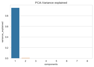
PCA 방법

components = 8
pca = PCA(n_components=components).fit(X)

pca_variance_explained_df = pd.DataFrame({
    "components" : np.arange(1, components + 1),
    "variance_explained" : pca.explained_variance_ratio_
})

ax = sns.barplot(x= 'components', y = 'variance_explained', data=pca_variance_explained_df)
ax.set_title("PCA-Variance explained")
plt.show()

농구_68_0

모델링 및 평가하기

X.head(3)

	action_type#Driving Layup Shot	action_type#Jump Shot	action_type#Layup Shot	combined_shot_type#Dunk	combined_shot_type#Jump Shot	combined_shot_type#Layup	game_month#1	game_month#11	game_month#12	game_month#2	game_month#3	game_month#4	home_away	loc_x#(-10.96, 8.96]	loc_y#(-10.6, 22.8]	loc_y#(123.0, 156.4]	loc_y#(22.8, 56.2]	opponent#SAS	period#1	period#2	period#3	period#4	playoffs	shot_distance	shot_type#2PT Field Goal	shot_type#3PT Field Goal	shot_zone_area#Center(C)	shot_zone_area#Left Side Center(LC)	shot_zone_area#Left Side(L)	shot_zone_area#Right Side Center(RC)	shot_zone_area#Right Side(R)	shot_zone_basic#Above the Break 3	shot_zone_basic#In The Paint (Non-RA)	shot_zone_basic#Mid-Range	shot_zone_basic#Restricted Area	shot_zone_range#16-24 ft.	shot_zone_range#24+ ft.	shot_zone_range#8-16 ft.	shot_zone_range#Less Than 8 ft.
shot_id
2	0	1	0	0	1	0	0	0	0	0	0	0	0	0	1	0	0	0	1	0	0	0	0	15	1	0	0	0	1	0	0	0	0	1	0	0	0	1	0
3	0	1	0	0	1	0	0	0	0	0	0	0	0	0	0	1	0	0	1	0	0	0	0	16	1	0	0	1	0	0	0	0	0	1	0	1	0	0	0
4	0	1	0	0	1	0	0	0	0	0	0	0	0	0	0	0	0	0	1	0	0	0	0	22	1	0	0	0	0	1	0	0	0	1	0	1	0	0	0

X.shape

(25697, 39)

Y.head(3)

shot_id
2    0.0
3    1.0
4    0.0
Name: shot_made_flag, dtype: category
Categories (2, float64): [0.0, 1.0]

Y.shape

(25697,)

## 각 알고리즘 및 함수의 configuration

seed=7
processors=1
num_folds=5
num_instance=len(X)
scoring='neg_log_loss'

k_fold = KFold(n_splits=num_folds, random_state = seed)

models = []
models.append(('LR', LogisticRegression()))
models.append(('LDA', LinearDiscriminantAnalysis()))
# knn은 근처에 몇개를 볼건지 알려줘야한다
models.append(('kNN',KNeighborsClassifier(n_neighbors=5)))
models.append(('CART',DecisionTreeClassifier()))

results = []
names = []

for name, model in models:
    cv_results = cross_val_score(model, X, Y, cv=k_fold, scoring = scoring, n_jobs=processors)
    results.append(cv_results)
    names.append(name)
    
    print('{}: {} +/- {}'.format(name, cv_results.mean(), cv_results.std()))

LR: -0.6188193218725694 +/- 0.004363985247902272
LDA: -0.6200222598834624 +/- 0.005268337905436931
kNN: -2.0409667268360083 +/- 0.1992975377549342
CART: -9.54050070397854 +/- 0.760930167111565

import sklearn
sklearn.metrics.SCORERS.keys()

dict_keys(['explained_variance', 'r2', 'max_error', 'neg_median_absolute_error', 'neg_mean_absolute_error', 'neg_mean_squared_error', 'neg_mean_squared_log_error', 'neg_root_mean_squared_error', 'neg_mean_poisson_deviance', 'neg_mean_gamma_deviance', 'accuracy', 'roc_auc', 'roc_auc_ovr', 'roc_auc_ovo', 'roc_auc_ovr_weighted', 'roc_auc_ovo_weighted', 'balanced_accuracy', 'average_precision', 'neg_log_loss', 'neg_brier_score', 'adjusted_rand_score', 'homogeneity_score', 'completeness_score', 'v_measure_score', 'mutual_info_score', 'adjusted_mutual_info_score', 'normalized_mutual_info_score', 'fowlkes_mallows_score', 'precision', 'precision_macro', 'precision_micro', 'precision_samples', 'precision_weighted', 'recall', 'recall_macro', 'recall_micro', 'recall_samples', 'recall_weighted', 'f1', 'f1_macro', 'f1_micro', 'f1_samples', 'f1_weighted', 'jaccard', 'jaccard_macro', 'jaccard_micro', 'jaccard_samples', 'jaccard_weighted'])

Ensemble(앙상블) 모형

다양한 모형의 예측 결과를 결합하여 사용하는 모형(여러 알고리즘을 결합하여 사용)
각각의 알고리즘은 상호 독립적이어야 하고, 오류 분류율은 적어도 50% 이상

Bagging

bootstrap Aggregation
- 통계적 분류와 회귀 분석에서 사용되는 기계학습 알고리즘의 안정성과 정확도를 향상시키기 위한 앙상블 학습법의 알고리즘
- 분산을 줄이고, overfitting을 피하도록 해준다.
- 주로, Decision Tree와 RandomForest에 적용

Decision Tree

cart = DecisionTreeClassifier()
num_trees = 100

model = BaggingClassifier(base_estimator=cart, n_estimators=num_trees, random_state=seed)

results = cross_val_score(model, X, Y, cv=k_fold, scoring = scoring, n_jobs=processors)

print('{} +/- {}'.format(results.mean(), results.std()))

-0.9178356241773005 +/- 0.02955286001580283

RandomForest

Bagging 종류 알고리즘 중 하나로 성능이 좋은 편

num_trees = 100
num_features = 10

model = RandomForestClassifier(n_estimators=num_trees, max_features=num_features)

results = cross_val_score(model, X, Y, cv=k_fold, scoring = scoring, n_jobs=processors)

print('{} +/- {}'.format(results.mean(), results.std()))

-0.9050138346040715 +/- 0.036967097078068625

Voting

estimators = []
# 여러 모델을 학습시키고 조합

estimators.append(('lr', LogisticRegression()))
estimators.append(('LDA',LinearDiscriminantAnalysis()))

ensemble = VotingClassifier(estimators, voting='soft', weights=[6,4])
results = cross_val_score(ensemble, X, Y, scoring=scoring, n_jobs=processors)

print('{} +/- {}'.format(results.mean(), results.std()))

-0.6195021443080785 +/- 0.007836031395028803

model = ensemble

import datetime
model.fit(X, Y)
preds = model.predict_proba(data_submit)

submission = pd.DataFrame()
submission['shot_id'] = data_submit.index
submission['shot_made_flag'] = preds[:,0]

submission.to_csv('sub_now.csv', index=False)

점수 높여보기

# 평가함수를 미리 만들어 본다
test_data = train[['loc_x', 'loc_y','shot_made_flag']]

test_data = test_data.dropna()

def test_it(data):
    clf = RandomForestClassifier(n_jobs=-1)
    return cross_val_score(clf, data.drop('shot_made_flag',1),data.shot_made_flag, scoring = 'neg_log_loss', cv = 10)

test_it(test_data).mean()

-0.8847544750995745

data = train[['loc_y','shot_made_flag']]
data = data.dropna()

test_it(data).mean()
# feature끼리 조합이 좋아야 학습이 잘된다

-0.6905886020233778

data = train[['shot_distance','shot_made_flag']]
data = data.dropna()

test_it(data).mean()

-0.6713330908479926

data = train[['shot_distance','loc_y','shot_made_flag']]
data = data.dropna()

test_it(data).mean()

-0.984015188449691

data = train[['seconds_remaining','shot_distance','shot_made_flag']]
data = data.dropna()

test_it(data).mean()

-0.8162567982043301

print(train.season.unique())

[2000-01, 2001-02, 2002-03, 2003-04, 2004-05, ..., 2015-16, 1996-97, 1997-98, 1998-99, 1999-00]
Length: 20
Categories (20, object): [2000-01, 2001-02, 2002-03, 2003-04, ..., 1996-97, 1997-98, 1998-99, 1999-00]

train['season_start_year'] = train.season.str.split('-').str[0]
train['seacon_start_year'] = train['season_start_year'].astype(int)

data = train[['seacon_start_year','shot_distance','shot_made_flag']]
data = data.dropna()

test_it(data).mean()

-1.2204021155277265

action_map = {action: i for i , action in enumerate(train.action_type.unique())}
train['action_type_enumerated'] = train.action_type.map(action_map)
train['action_type_enumerated']

shot_id
      0
      0
      0
      1
      0
        ..
  6
  0
  3
  0
  0
Name: action_type_enumerated, Length: 25697, dtype: int64

data = train[['action_type_enumerated','shot_distance','shot_made_flag']]
data = data.dropna()

test_it(data).mean()

-0.6497893336065241

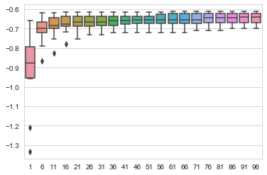
data = train[['action_type_enumerated','shot_distance','shot_made_flag']].dropna()

estimators, scores = list(range(1,100,5)), []

for i in estimators:
    clf = RandomForestClassifier(n_jobs=-1, n_estimators=i, random_state=2016)
    x = cross_val_score(clf, data.drop(['shot_made_flag'],1), data.shot_made_flag, scoring='neg_log_loss', cv = 10)
    scores.append(x)
    
x = [i for i in estimators for j in range(10)]
sns.boxplot(x, np.array(scores).flatten())

<matplotlib.axes._subplots.AxesSubplot at 0x179001e5688>

농구_102_1

depth, scores = list(range(1,20,1)), []

for i in depth:
    clf = RandomForestClassifier(n_jobs=-1, n_estimators=70,max_depth=i, random_state=2016)
    x = cross_val_score(clf, data.drop(['shot_made_flag'],1), data.shot_made_flag, scoring='neg_log_loss', cv = 10)
    scores.append(x)
    
x = [i for i in depth for j in range(10)]
sns.boxplot(x, np.array(scores).flatten())

<matplotlib.axes._subplots.AxesSubplot at 0x179019cf908>

농구_103_1

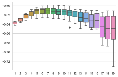
clf = RandomForestClassifier(n_jobs=-1, n_estimators=70, max_depth=7, random_state=2016) # a more powerful classifier

train_data = train.loc[~train.shot_made_flag.isnull(), ['action_type_enumerated',
                                             'shot_distance', 'shot_made_flag', 'away']]
test = train.loc[train.shot_made_flag.isnull(), ['action_type_enumerated',
                                           'shot_distance', 'shot_id', 'away']]
# Impute
mode = test.action_type_enumerated.mode()[0]
test.action_type_enumerated.fillna(mode, inplace=True)

# Train and predict
clf.fit(train_data.drop('shot_made_flag', 1), train_data.shot_made_flag)
predictions = clf.predict_proba(test.drop('shot_id', 1))

import datetime
submission = pd.DataFrame({'shot_id': test.shot_id,
                           'shot_made_flag': predictions[:, 1]})
submission[['shot_id', 'shot_made_flag']].to_csv('submission{}.csv'.format(datetime.datetime.now()), index=False)

Share on

Twitter Facebook LinkedIn

Lim Junhyeong

실습. 코비선수 데이터 분석해보기 및 테스트

데이터 분석

데이터 살펴보기

데이터 분석 및 시각화

Feature Engineering

Data cleaning

Data Transformation

중요 컬럼을 뽑아내기

분산을 이용

RandomForestClassifier 사용

PCA 방법

모델링 및 평가하기

Ensemble(앙상블) 모형

Bagging

Decision Tree

RandomForest

Voting

점수 높여보기

Share on

Leave a comment

You may also enjoy

mariaDB 환경설정 계정 생성 및 권한 부여

프로젝트에 필요한 Git

여러개의 원격 저장소(git)

벽 부수고 이동하기 4_16946