Pandas, Numpy, Matplotlib

Updated: July 09, 2020

벡터의 표현

import numpy as np 
a = np.array([2,1])
print(a)
​
b = np.array([3,2,1])
print(b)
​
A = np.array([[2,4,1],[6,3,5]])
print(A)
​
# 벡터는 numpy를 사용하여 나타낼수 있다

[2 1]
[3 2 1]
[[2 4 1]
[6 3 5]]

벡터의 기본 연산

import numpy as np
import math
​
a = np.array([3,2])
b = np.array([1,3])
​
print(a + b)
print(a - b)
# 벡터의 합과 차
​
print(np.linalg.norm(a))
print(np.linalg.norm(b))
# 벡터의 크기를 구하는 1번 방식
​
def norm(x):
    return math.sqrt(sum([i ** 2 for i in x]))
​
print(norm(a))
print(norm(b))
# 벡터의 크기를 구하는 2번 방식
​
# 벡터의 크기는 피타고라스 연산을 사용하여 구할수 있다.

[4 5]
[ 2 -1]
3.605551275463989
3.1622776601683795
3.605551275463989
3.1622776601683795

벡터의 내적

​
# 두 벡터가 수직일 때는 벡터의 내적은 항상 0입니다
# 내적이 양수 일때는 두 벡터가 이루는 각이 90도 보다 작고, 내적이 음수 일때는 
# 두 벡터가 이루는 각이 90도보다 커진다
​
import numpy as np
​
a = np.array([3,2])
b = np.array([1,4])
​
print(a.dot(b))
​
c = np.array([2,1])
d = np.array([-1,2])
​
print(c.dot(d))
# dot을 사용하여 두 벡터의 내적을 구할 수 있다
# 두 벡터 a, b의 방향이 같을 때 내적을 계산하면 |a||b|고 내적의 최댓값이다
# 두 벡터 a, b의 방향이 반대일 때 내적을 계산하면 -|a||b|고 내적의 최솟값이다
# 두 벡터가 이루는 방향으로 내적이 최댓값인지 최솟값인지 알 수 있다
​
# 이는 신경망에서 최솟값을 계산하고 싶을 때 응용된다

11
0

행렬의 덧셈과 뺄셈

import numpy as np
​
X = np.array([[1,2,3],[3,4,5]])
Y = np.array([[3,4,5],[4,5,6]])
​
print(X + Y)
print(X - Y)

[[ 4 6 8]
[ 7 9 11]]
[[-2 -2 -2]
[-1 -1 -1]]

행렬의 곱셈

# m * k행렬과 k * n행렬의 결과는 m * n행렬이 나온다
​
import numpy as np
​
A = np.array([[[1,2,3],[3,4,5]]])
B = np.array([[3,4],[4,5],[5,6]])
​
print(A.dot(B))
​
C = np.matrix([[1,2,3],[3,4,5]])
D = np.matrix([[3,4],[4,5],[5,6]])
​
# matrix를 사용해서 행렬을 만들수 있다
# 행렬은 교환법칙이 성립하지 않는다. AB != BA
print(C * D)

[[[26 32]
[50 62]]]
[[26 32]
[50 62]]

단위행렬

# 대각선 원소가 1이고 나머지 원소가 0인 행렬
# E로 표현

전치행렬

# 행렬의 행과 열을 교환한 행렬
# 전치행렬의 전치행렬은 원래의 행렬 
# T를 사용하여 표현

역행렬

# AB가 E(단위행렬)이면 B를 A의 역행렬이라고 하고 A^-1로 표현한다
​
import numpy as np
A = np.array([[2,5],[1,3]])
​
print(np.linalg.inv(A))
# 역행렬을 구하는법

[[ 3. -5.]
[-1. 2.]]

Pandas

# 데이터를 불러올수 있다
​
# 경로 설정이 어려울 경우 경로를 확인할 수 있다
import os
print(os.getcwd())

C:\Users\user\Desktop\인공지능사관

## 출력확인
import pandas as pd
df = pd.read_csv('gapminder.tsv',sep='\t')
print(df.head())

country continent year lifeExp pop gdpPercap
0 Afghanistan Asia 1952 28.801 8425333 779.445314
1 Afghanistan Asia 1957 30.332 9240934 820.853030
2 Afghanistan Asia 1962 31.997 10267083 853.100710
3 Afghanistan Asia 1967 34.020 11537966 836.197138
4 Afghanistan Asia 1972 36.088 13079460 739.981106

변수 타입확인

print(type(df))

데이터의 행렬 크기 확인

print(df.shape)

(1704, 6)

데이터의 컬럼값 확인

print(df.columns)

Index([‘country’, ‘continent’, ‘year’, ‘lifeExp’, ‘pop’, ‘gdpPercap’], dtype=’object’)

데이터 타입확인

print(df.dtypes)

country object
continent object
year int64
lifeExp float64
pop int64
gdpPercap float64
dtype: object

열 단위로 데이터 추출하기

country_df = df['country']
print(country_df.head())
print(country_df.tail())

0 Afghanistan
1 Afghanistan
2 Afghanistan
3 Afghanistan
4 Afghanistan
Name: country, dtype: object

1699 Zimbabwe
1700 Zimbabwe
1701 Zimbabwe
1702 Zimbabwe
1703 Zimbabwe
Name: country, dtype: object

여러 열 단위 추출하기

subset = df[['country','continent','year']]
print(subset.head())
print(subset.tail())

country continent year
0 Afghanistan Asia 1952
1 Afghanistan Asia 1957
2 Afghanistan Asia 1962
3 Afghanistan Asia 1967
4 Afghanistan Asia 1972

country continent year
1699 Zimbabwe Africa 1987
1700 Zimbabwe Africa 1992
1701 Zimbabwe Africa 1997
1702 Zimbabwe Africa 2002
1703 Zimbabwe Africa 2007

loc 속성으로 행 데이터 추출하기

print(df.loc[0])
print(df.loc[99])

country Afghanistan
continent Asia
year 1952
lifeExp 28.801
pop 8425333
gdpPercap 779.445
Name: 0, dtype: object

country Bangladesh
continent Asia
year 1967
lifeExp 43.453
pop 62821884
gdpPercap 721.186
Name: 99, dtype: object

마지막 행 데이터 추출하기

print(df.tail(n=1))

country continent year lifeExp pop gdpPercap
1703 Zimbabwe Africa 2007 43.487 12311143 469.709298

원하는 다중 행 출력하기

print(df.loc[[0,99,999]])

country continent year lifeExp pop gdpPercap
0 Afghanistan Asia 1952 28.801 8425333 779.445314
99 Bangladesh Asia 1967 43.453 62821884 721.186086
999 Mongolia Asia 1967 51.253 1149500 1226.041130

데이터 행 추출

print(df.iloc[1])
print(df.iloc[99])
print(df.iloc[-1])

country Afghanistan
continent Asia
year 1957
lifeExp 30.332
pop 9240934
gdpPercap 820.853
Name: 1, dtype: object

country Bangladesh
continent Asia
year 1967
lifeExp 43.453
pop 62821884
gdpPercap 721.186
Name: 99, dtype: object

country Zimbabwe
continent Africa
year 2007
lifeExp 43.487
pop 12311143
gdpPercap 469.709
Name: 1703, dtype: object

슬라이싱을 활용한 데이터 추출 (변수명)

subset = df.loc[:, ['year','pop']]
print(subset.head())

year pop
0 1952 8425333
1 1957 9240934
2 1962 10267083
3 1967 11537966
4 1972 13079460

슬라이싱을 활용한 데이터 추출 (정수)

subset = df.iloc[:, [2,4,-1]]
print(subset.head())

year pop gdpPercap
0 1952 8425333 779.445314
1 1957 9240934 820.853030
2 1962 10267083 853.100710
3 1967 11537966 836.197138
4 1972 13079460 739.981106

다양한 방식의 데이터 추출

print(df.iloc[[0,99,999],[0,3,5]])
print(df.loc[[0,99,999],['country', 'lifeExp','gdpPercap']])

country lifeExp gdpPercap
0 Afghanistan 28.801 779.445314
99 Bangladesh 43.453 721.186086
999 Mongolia 51.253 1226.041130
country lifeExp gdpPercap
0 Afghanistan 28.801 779.445314
99 Bangladesh 43.453 721.186086
999 Mongolia 51.253 1226.041130

# groupby를 활용한 그룹화한 데이터 기초 통계자산
# (연도별) [기대수명]의 평균 구하기
# (그룹화) [구하고자 하는 값]
print(df.groupby('year')['lifeExp'].mean())

year
1952 49.057620
1957 51.507401
1962 53.609249
1967 55.678290
1972 57.647386
1977 59.570157
1982 61.533197
1987 63.212613
1992 64.160338
1997 65.014676
2002 65.694923
2007 67.007423
Name: lifeExp, dtype: float64

# ([연도명, 대륙별])[[기대수명, 1인 gdp]]의 평균 구하기
# (그룹화) [구하고자 하는 값]
print(df.groupby(['year','continent'])[['lifeExp','gdpPercap']].mean())

year continent lifeExp gdpPercap

1952 Africa 39.135500 1252.572466
Americas 53.279840 4079.062552
Asia 46.314394 5195.484004
Europe 64.408500 5661.057435
Oceania 69.255000 10298.085650
1957 Africa 41.266346 1385.236062
Americas 55.960280 4616.043733
Asia 49.318544 5787.732940
Europe 66.703067 6963.012816
Oceania 70.295000 11598.522455
1962 Africa 43.319442 1598.078825
Americas 58.398760 4901.541870
Asia 51.563223 5729.369625
Europe 68.539233 8365.486814
Oceania 71.085000 12696.452430
1967 Africa 45.334538 2050.363801
Americas 60.410920 5668.253496
Asia 54.663640 5971.173374
Europe 69.737600 10143.823757
Oceania 71.310000 14495.021790
1972 Africa 47.450942 2339.615674
Americas 62.394920 6491.334139
Asia 57.319269 8187.468699
Europe 70.775033 12479.575246
Oceania 71.910000 16417.333380
1977 Africa 49.580423 2585.938508
Americas 64.391560 7352.007126
Asia 59.610556 7791.314020
Europe 71.937767 14283.979110
Oceania 72.855000 17283.957605
1982 Africa 51.592865 2481.592960
Americas 66.228840 7506.737088
Asia 62.617939 7434.135157
Europe 72.806400 15617.896551
Oceania 74.290000 18554.709840
1987 Africa 53.344788 2282.668991
Americas 68.090720 7793.400261
Asia 64.851182 7608.226508
Europe 73.642167 17214.310727
Oceania 75.320000 20448.040160
1992 Africa 53.629577 2281.810333
Americas 69.568360 8044.934406
Asia 66.537212 8639.690248
Europe 74.440100 17061.568084
Oceania 76.945000 20894.045885
1997 Africa 53.598269 2378.759555
Americas 71.150480 8889.300863
Asia 68.020515 9834.093295
Europe 75.505167 19076.781802
Oceania 78.190000 24024.175170
2002 Africa 53.325231 2599.385159
Americas 72.422040 9287.677107
Asia 69.233879 10174.090397
Europe 76.700600 21711.732422
Oceania 79.740000 26938.778040
2007 Africa 54.806038 3089.032605
Americas 73.608120 11003.031625
Asia 70.728485 12473.026870
Europe 77.648600 25054.481636
Oceania 80.719500 29810.188275

그룹화한 데이터의 개수 즉, 빈도수 구하기

# (대륙별) [나라].빈도수 확인()
print(df.groupby('continent')['country'].nunique())

continent
Africa 52
Americas 25
Asia 33
Europe 30
Oceania 2
Name: country, dtype: int64

matplotlib.pyplot

matplotlib.pyplot 호출

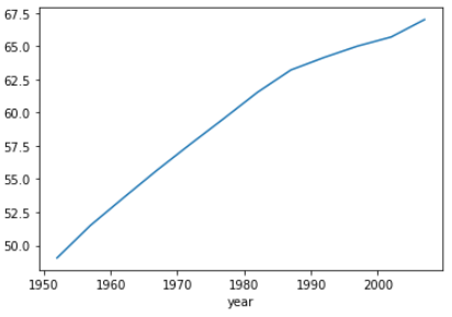
import matplotlib.pyplot as plt
​
# (연도별)[기대수명] 평균내어 변수화
global_yearly_life_expectancy = df.groupby('year')['lifeExp'].mean()
​
# 출력
print(global_yearly_life_expectancy)
​
# 그래프 출력
global_yearly_life_expectancy.plot()
plt.show()

global_year_life

데이터프레임 만들기

corona_data = pd.DataFrame(
    # 실질적으로 들어가게 될 데이터, 컬럼명 : [데이터들]
    data = {'city' : ['seoul','gyeong-gi'],
           'patient':[1580,1300],
           'today_parient' : [15,10],
           'date' : ['2020-07-09','2020-07-09']},
    # 인덱스 설정
    index = ['seoul','gyeong-gi'],
    # 컬럼명 설정
    columns = ['patient','today_parient','date'])
​
# 출력
print(corona_data)

patient today_parient date
seoul 1580 15 2020-07-09
gyeong-gi 1300 10 2020-07-09

행 위주의 출력

seoul = corona_data.loc['seoul']
print(seoul)
print(seoul.index)
print(seoul.values)

patient 1580
today_parient 15
date 2020-07-09
Name: seoul, dtype: object

Index([‘patient’, ‘today_parient’, ‘date’], dtype=’object’)

[1580 15 ‘2020-07-09’]

scientists = pd.read_csv('scientists.csv')
scientists.head()
​
# 브로드 캐스팅 : 데이터 프레임에 있는 모든 데이터에 대해 한번에 연산하는 것
​
# 변수선택[행추출['컬럼지정'] > ['컬럼지정'].mean()]
print(scientists[scientists['Age'] > scientists['Age'].mean()])

Name Born Died Age Occupation
1 William Gosset 1876-06-13 1937-10-16 61 Statistician
2 Florence Nightingale 1820-05-12 1910-08-13 90 Nurse
3 Marie Curie 1867-11-07 1934-07-04 66 Chemist
7 Johann Gauss 1777-04-30 1855-02-23 77 Mathematician

시리즈와 데이터프레임처리

born_datetime = pd.to_datetime(scientists['Born'], format = '%Y-%m-%d')
print(born_datetime)
died_datetime = pd.to_datetime(scientists['Died'], format = '%Y-%m-%d')
print(died_datetime)

0 1920-07-25
1 1876-06-13
2 1820-05-12
3 1867-11-07
4 1907-05-27
5 1813-03-15
6 1912-06-23
7 1777-04-30
Name: Born, dtype: datetime64[ns]

0 1958-04-16
1 1937-10-16
2 1910-08-13
3 1934-07-04
4 1964-04-14
5 1858-06-16
6 1954-06-07
7 1855-02-23
Name: Died, dtype: datetime64[ns]

# 변수['새로운 컬럼할당','새로운 컴럼할당'] = (시계열데이터, 시계열 데이터)  
scientists['born_dt'], scientists['died_dt'] = (born_datetime , died_datetime)
print(scientists.head())

Name Born Died Age Occupation born_dt \
0 Rosaline Franklin 1920-07-25 1958-04-16 37 Chemist 1920-07-25
1 William Gosset 1876-06-13 1937-10-16 61 Statistician 1876-06-13
2 Florence Nightingale 1820-05-12 1910-08-13 90 Nurse 1820-05-12
3 Marie Curie 1867-11-07 1934-07-04 66 Chemist 1867-11-07
4 Rachel Carson 1907-05-27 1964-04-14 56 Biologist 1907-05-27

died_dt
0 1958-04-16
1 1937-10-16
2 1910-08-13
3 1934-07-04
4 1964-04-14

# 새로운 컬럼에 할당 - 시계열 - 시계열
scientists['age_days_dt'] = (scientists['died_dt'] - scientists['born_dt'])
print(scientists)

Name Born Died Age Occupation \
0 Rosaline Franklin 1920-07-25 1958-04-16 37 Chemist
1 William Gosset 1876-06-13 1937-10-16 61 Statistician
2 Florence Nightingale 1820-05-12 1910-08-13 90 Nurse
3 Marie Curie 1867-11-07 1934-07-04 66 Chemist
4 Rachel Carson 1907-05-27 1964-04-14 56 Biologist
5 John Snow 1813-03-15 1858-06-16 45 Physician
6 Alan Turing 1912-06-23 1954-06-07 41 Computer Scientist
7 Johann Gauss 1777-04-30 1855-02-23 77 Mathematician

born_dt died_dt age_days_dt
0 1920-07-25 1958-04-16 13779 days
1 1876-06-13 1937-10-16 22404 days
2 1820-05-12 1910-08-13 32964 days
3 1867-11-07 1934-07-04 24345 days
4 1907-05-27 1964-04-14 20777 days
5 1813-03-15 1858-06-16 16529 days
6 1912-06-23 1954-06-07 15324 days
7 1777-04-30 1855-02-23 28422 days

Share on

Twitter Facebook LinkedIn

Lim Junhyeong