
시각화(matplotlib)
Updated:
기본셋팅
import matplotlib.pyplot as plt
import seaborn as sns
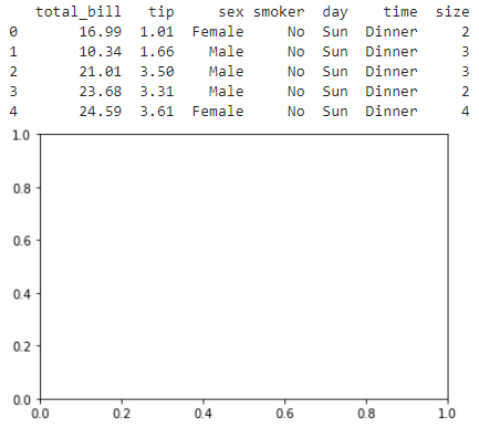
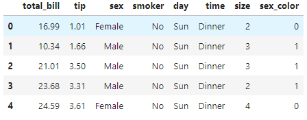
# tips데이터 불러오기 및 저장
# 손님들이 지불한 tip정보
tips = sns.load_dataset("tips")
print(tips.head())
# 번 그래프 그리기
fig = plt.figure()
# add_subplot(행 크기, 열 크기, 들어갈 위치)
axes1 = fig.add_subplot(1,1,1)
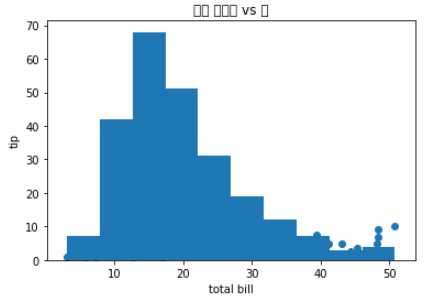
히스토그램
# 히스토그램 분포도
# hist(변수['컬럼'], x축 간격 10)
axes1.hist(tips['total_bill'], bins = 10)
# 상단의 이름
axes1.set_title('Histogram of total Bill')
# x축의 이름
axes1.set_xlabel('Frequency')
# y축의 이름
axesl.set_ylabel('Total Bill')
fig
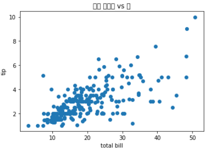
산점도 그래프
# 기본 틀 생성
scatter_plot = plt.figure()
# 그래프 격자 생성
axes1 = scatter_plot.add_subplot(1,1,1)
# scatter(변수[컬럼_1 : total_bill], 변수[컬럼_2:tip])
axes1.scatter(tips['total_bill'],tips['tip'])
axes1.set_title('전체 지불액 vs 팁') # 한글은 잘 적용되지 않는다.
axes1.set_xlabel('total bill')
axes1.set_ylabel('tip')
plt.show()
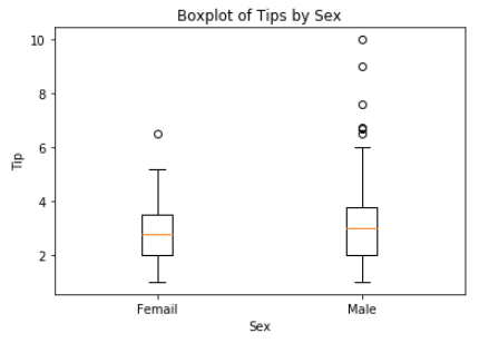
박스 그래프
# 기본 틀 생선
boxplot = plt.figure()
# 격자 생성
axes1 = boxplot.add_subplot(1,1,1)
# tips데이터 프레임에서 성별이 남자와 여자인 데이터에서 tips 열 데이터만 추출하여
# 리스트에 담아 전달
# 데이터프레임[데이터 프레임내의 ['컬럼명'] == ['femail'][열 선택 추출]]
axes1.boxplot([tips[tips['sex'] == 'Female']['tip'],
tips[tips['sex'] == 'Male']['tip']],
labels = ['Femail','Male'])
axes1.set_xlabel('Sex')
axes1.set_ylabel('Tip')
axes1.set_title('Boxplot of Tips by Sex')
plt.show()
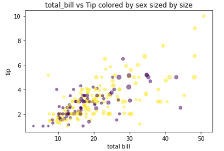
다변량 그래프
# 문자열 데이터 치환과정 male, female -> 남자_1, 여자_0
def recode_sex(sex):
if sex == 'Female':
return 0
else:
return 1
# apply함수활용
# tips['sex_color'] 새로운 컴럼 생성 = tips의 ['sex']에.함수적용(자체함수)
tips['sex_color'] = tips['sex'].apply(recode_sex)
tips.head()# 새로운 변수 확인
scatter_plot = plt.figure()
axes1 = scatter_plot.add_subplot(1,1,1)
axes1.scatter(
x = tips['total_bill'],
y = tips['tip'],
s = tips['size'] * 10, # s는 점의 크기를 할당, 점의 크기를 인원수로 설정
c = tips['sex_color'], # c는 생상을 할당, 남자, 여자로 분리하여 할당
alpha = 0.5) # 투명도
axes1.set_title('total_bill vs Tip colored by sex sized by size')
axes1.set_xlabel('total bill')
axes1.set_ylabel('tip')
plt.show()
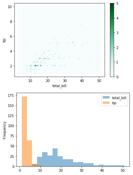
산점도
fig, ax = plt.subplots()
ax = tips.plot.hexbin(x = 'total_bill', y = 'tip', ax = ax)
# 히스토그램
fig, ax = plt.subplots()
ax = tips[['total_bill', 'tip']].plot.hist(alpha = 0.5, bins = 20, ax = ax)
결측치
from numpy import NaN, NAN, nan
# isnull을 통해 결측값 검사
print(pd.isnull((NaN)))
print(pd.isnull((nan)))
print(pd.isnull((NAN)))
visited = pd.read_csv('survey_visited.csv')
survey = pd.read_csv('survey_survey.csv')
print(visited)
print(survey)
True
True
True
ident site dated
0 619 DR-1 1927-02-08
1 622 DR-1 1927-02-10
2 734 DR-3 1939-01-07
3 735 DR-3 1930-01-12
4 751 DR-3 1930-02-26
5 752 DR-3 NaN
6 837 MSK-4 1932-01-14
7 844 DR-1 1932-03-22
taken person quant reading
0 619 dyer rad 9.82
1 619 dyer sal 0.13
2 622 dyer rad 7.80
3 622 dyer sal 0.09
4 734 pb rad 8.41
5 734 lake sal 0.05
6 734 pb temp -21.50
7 735 pb rad 7.22
8 735 NaN sal 0.06
9 735 NaN temp -26.00
10 751 pb rad 4.35
11 751 pb temp -18.50
12 751 lake sal 0.10
13 752 lake rad 2.19
14 752 lake sal 0.09
15 752 lake temp -16.00
16 752 roe sal 41.60
17 837 lake rad 1.46
18 837 lake sal 0.21
19 837 roe sal 22.50
20 844 roe rad 11.25
# 데이터 결합을 위한 merge()
vs = visited.merge(survey, left_on='ident', right_on = 'taken')
print(vs)
print(vs.count()) #열 별로 결측값 출력
print("==========================================================")
# 결측값 삭제하기
vs_dropna = vs.dropna()
print(vs_dropna)
print("==========================================================")
# 결측값 0 처리
vs_fillna = vs.fillna(0)
print(vs_fillna)
ident site dated taken person quant reading
0 619 DR-1 1927-02-08 619 dyer rad 9.82
1 619 DR-1 1927-02-08 619 dyer sal 0.13
2 622 DR-1 1927-02-10 622 dyer rad 7.80
3 622 DR-1 1927-02-10 622 dyer sal 0.09
4 734 DR-3 1939-01-07 734 pb rad 8.41
5 734 DR-3 1939-01-07 734 lake sal 0.05
6 734 DR-3 1939-01-07 734 pb temp -21.50
7 735 DR-3 1930-01-12 735 pb rad 7.22
8 735 DR-3 1930-01-12 735 NaN sal 0.06
9 735 DR-3 1930-01-12 735 NaN temp -26.00
10 751 DR-3 1930-02-26 751 pb rad 4.35
11 751 DR-3 1930-02-26 751 pb temp -18.50
12 751 DR-3 1930-02-26 751 lake sal 0.10
13 752 DR-3 NaN 752 lake rad 2.19
14 752 DR-3 NaN 752 lake sal 0.09
15 752 DR-3 NaN 752 lake temp -16.00
16 752 DR-3 NaN 752 roe sal 41.60
17 837 MSK-4 1932-01-14 837 lake rad 1.46
18 837 MSK-4 1932-01-14 837 lake sal 0.21
19 837 MSK-4 1932-01-14 837 roe sal 22.50
20 844 DR-1 1932-03-22 844 roe rad 11.25
ident 21
site 21
dated 17
taken 21
person 19
quant 21
reading 21
dtype: int64
ident site dated taken person quant reading
0 619 DR-1 1927-02-08 619 dyer rad 9.82
1 619 DR-1 1927-02-08 619 dyer sal 0.13
2 622 DR-1 1927-02-10 622 dyer rad 7.80
3 622 DR-1 1927-02-10 622 dyer sal 0.09
4 734 DR-3 1939-01-07 734 pb rad 8.41
5 734 DR-3 1939-01-07 734 lake sal 0.05
6 734 DR-3 1939-01-07 734 pb temp -21.50
7 735 DR-3 1930-01-12 735 pb rad 7.22
10 751 DR-3 1930-02-26 751 pb rad 4.35
11 751 DR-3 1930-02-26 751 pb temp -18.50
12 751 DR-3 1930-02-26 751 lake sal 0.10
17 837 MSK-4 1932-01-14 837 lake rad 1.46
18 837 MSK-4 1932-01-14 837 lake sal 0.21
19 837 MSK-4 1932-01-14 837 roe sal 22.50
20 844 DR-1 1932-03-22 844 roe rad 11.25
ident site dated taken person quant reading
0 619 DR-1 1927-02-08 619 dyer rad 9.82
1 619 DR-1 1927-02-08 619 dyer sal 0.13
2 622 DR-1 1927-02-10 622 dyer rad 7.80
3 622 DR-1 1927-02-10 622 dyer sal 0.09
4 734 DR-3 1939-01-07 734 pb rad 8.41
5 734 DR-3 1939-01-07 734 lake sal 0.05
6 734 DR-3 1939-01-07 734 pb temp -21.50
7 735 DR-3 1930-01-12 735 pb rad 7.22
8 735 DR-3 1930-01-12 735 0 sal 0.06
9 735 DR-3 1930-01-12 735 0 temp -26.00
10 751 DR-3 1930-02-26 751 pb rad 4.35
11 751 DR-3 1930-02-26 751 pb temp -18.50
12 751 DR-3 1930-02-26 751 lake sal 0.10
13 752 DR-3 0 752 lake rad 2.19
14 752 DR-3 0 752 lake sal 0.09
15 752 DR-3 0 752 lake temp -16.00
16 752 DR-3 0 752 roe sal 41.60
17 837 MSK-4 1932-01-14 837 lake rad 1.46
18 837 MSK-4 1932-01-14 837 lake sal 0.21
19 837 MSK-4 1932-01-14 837 roe sal 22.50
20 844 DR-1 1932-03-22 844 roe rad 11.25
Leave a comment